Plate-Heat-Exchangers
Overview and Geometry
The motivating factor that drives the use of brazed-plate heat exchangers is that they are a highly-compact heat exchanger that allows for excellent heat transfer between two fluids with very well controlled pressure drop. They tend to be slightly more expensive than equivalent coaxial type heat exchangers due to their more exacting manufacturing requirements. But they can be easily altered to add more plates to give more surface area for increased heat transfer area and lower pressure drop. The trade-off as usual is that adding plates to decrease the pressure drop also results in a decrease in heat transfer coefficient, which means that each m2 of surface area in the HX becomes less useful.
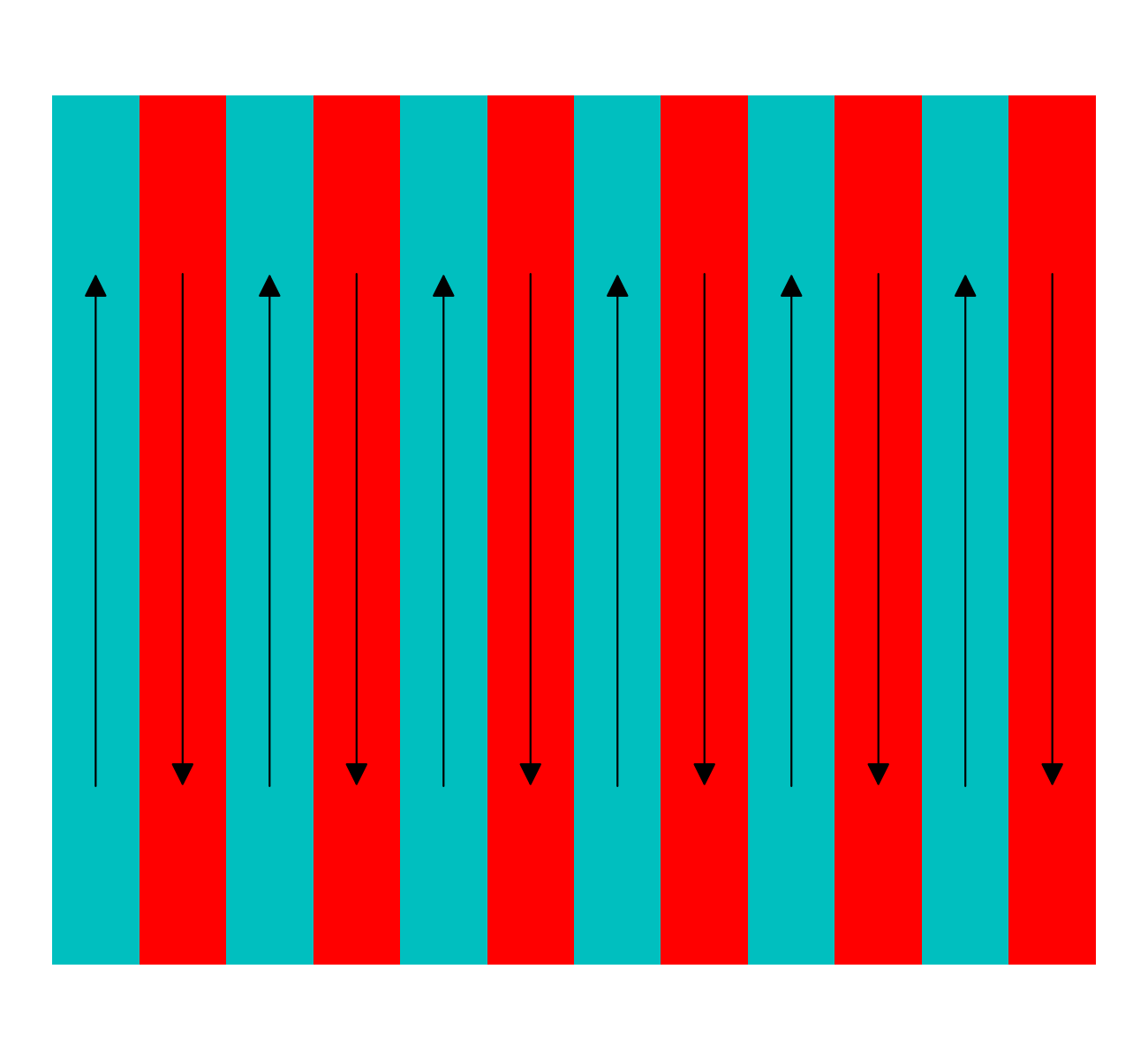
In the most basic configuration of a plate heat exchanger, hot and cold streams in pure counterflow alternate through the stack of plates. From the side view, a simplified schematic of the BPHE is something like this:
(Source code, png, hires.png, pdf)
In practice, it is sometimes useful to have one of the stream do multiple passes for one pass of the other stream, but this capability is not included in the BPHE model as of this time. This is commonly used when the capacitance rates are very different, a sufficient heat transfer rate cannot be achieved for one fluid, or when one of the fluids is particularly sensitive to pressure drop. All of these issues are particularly strongly felt for the flow of gases.
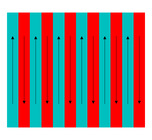
In practice, what you get when you put it all together is a heat exchanger that looks something like from face-on:
(Source code, png, hires.png, pdf)

Robust gasketing of the plates is required to ensure that the fluid phases do not mix at the inlets and outlets of the plates.
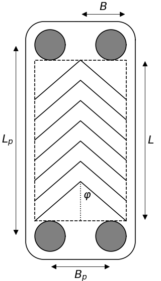
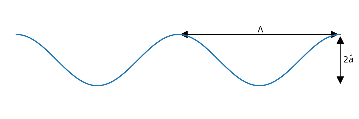
Each of the plates that form the internal surface of the BPHE are formed of plates with a wavy shape, and the edge of the plate looks something like this:
(Source code, png, hires.png, pdf)
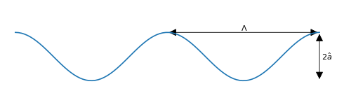
Based on this geometry, the hydraulic diameter \(d_h\) is defined by
where the parameter \(\Phi\) is the ratio of the actual area to the planar area enclosed by the edges of the plate (bounded by \(L\) and \(B\) in the figure above). Typically the plates do not have exactly a sinusoidal profile, but, to a decent approximation, their profile is sinusoidal, which results in the value of \(\Phi\) of
where the wavenumber \(X\) is given by
When the plates are put together to form a stack, the plates are alternated, and as a result, chevron-shaped flow paths are formed, which have the effect of yielding highly mixed flow, resulting in good heat transfer coefficients
A stack of \(N_{plates}\) plates form the heat exchanger. There are a total of \(N_{channels}\) channels formed between the plates. If \(N_{channels}\) is evenly divisible by 2, both fluids have the same number of channels. If \(N_{channels}\) is not evenly divisible by 2, one stram must have one extra channel. The outer two plates don’t provide any heat transfer as they are just used to maintain the channel structure for the outermost channels. There are therefore a total of \(N_{plates}-2\) active plates, for which the active area of one side of one plate is equal to
Each channel of a fluid gets two sides of this area, which yields the cold- and hot-side wetted areas of
and the mass flow rate of the hot and cold fluids per circuit (needed for correlations), is equal to
Heat Transfer and Pressure Drop Correlations
Single-Phase Flow
When there is single-phase flow on one side of the heat exchanger, the analysis of Martin [6] from the VDI Heat Atlas is employed. The nomenclature used here mirrors that of Martin. Using this analysis, the pressure drop and heat transfer coefficients for the fluid flowing between the plates can be calculated.
The Reynolds number for the flow through the channel between two plates is given by
where the velocity per channel is given by
The pressure drop and heat transfer coefficients are usual a function of the Reynolds number, and if the flow is laminar (\(\mathrm{Re}<2000\)), the factors \(\zeta_0\) and \(\zeta_{1,0}\) are given by
and if the flow is turbulent (\(\mathrm{Re}\geq 2000\)), the factors \(\zeta_0\) and \(\zeta_{1,0}\) are given by
The friction factor \(\zeta\) is obtained from
where the factor \(\zeta_1\) is given by
and the factors \(a\) and \(b\) and \(c\) given by Martin are
The Hagen number is defined by
which gives the value for the pressure drop
The Nusselt number is obtained from
where the recommended values of the constants \(c_q\) and \(q\) from Martin are 0.122 and 0.374 respectively. Finally the overall heat transfer coefficient is obtained from
Two-Phase Evaporating Flow
When the fluid flow is evaporating, it is quite a bit more difficult to determine the best model to use. There are contradictory conclusions drawn in literature as to what type of heat transfer is occurring.
It seems like the most accepted view, though is open to debate, is that the flow is governed by nucleate boiling within the channels, and as a result, nucleate pool boiling relations are employed in order to calculate the heat transfer coefficient. This model has some features which are not well-suited to implementation into the PHE model. For one, there is no quality dependence on heat transfer coefficient, which yields un-physically high values of heat transfer coefficient at high quality (should go to the saturated vapor gas heat transfer coefficient at pure vapor).
In spite of these shortcomings, the pool boiling correlation of Cooper [5] was used. This yields a simple form of the solution for the heat transfer coefficient. The heat transfer coefficient is obtained from
where
and \(M\) is the molar mass (kg/kmol) of the fluid and \(R_p\) is the relative roughness of the surface and K is set to unity. However, Claesson [4] suggested a correction of 1.5.
In order to calculate the pressure drop in evaporating flow in the PHE channel, the frictional pressure drop is calculated using the Lockhart-Martinelli two-phase pressure drop correlation from section Lockhart-Martinelli with the value of the parameter C of 4.67 as recommended by Claesson [4]. The accelerational pressure change is given from the same section.
Two-Phase Condensing Flow
The available models for condensing flow in PHE share many of the shortcomings of the evaporating flow models. There is a paucity of good data available, since most of the know-how is controlled by the major PHE manufacturers. That said, many researchers have studied this topic, but the parameter space (geometrically and thermodynamically) is quite vast. This is still a topic that could do with further study.
Longo has conducted studies [1] [2] [3] that looked at condensation in PHE, and from these studies it can be seen that at low equivalent Reynolds number (\(\mathrm{Re}_{eq}<1750\)), the j-factor is nominally constant at a value of 60, and above that, it is linear with equivalent Reynolds number, so the j-factor can be given by
where the equivalent Reynolds number is defined by
which finally yields the heat transfer coefficient
Mathematical Description
With the set of required correlations defined, it is now possible to analyze the plate heat exchanger for a range of different configurations. The PHE model is constructed to be general enough that it can handle any phase of fluids entering into the heat exchanger. The basic idea behind the PHE model is a two-step process:
- Determine the bounding heat transfer rate (100% effectiveness) limited by taking each fluid to the inlet temperature of the other fluid. This is the most amount of heat transfer possible. Also watch out for internal pinch points
- Since the heat transfer rate is now bounded between zero and the maximum, iterate to find the actual heat transfer rate in the heat exchanger in order to yield the “right-size” heat exchanger (see description below)
Bounds on Heat Transfer Rate
Since the PHE is pure counterflow, the coldest possible temperature that the hot stream can achieve is the inlet temperature of the cold stream, and similarly, the hottest temperature that the cold stream can achieve is the inlet temperature of the hot stream. The inlet enthalpies of the hot stream \(h_{h,i}\) and the cold stream \(h_{c,i}\) allow to calculate a preliminary value for the upper bound on the heat transfer rate:
Using this preliminary bound on the heat transfer rate, it is then possible to determine the enthalpies and temperatures of both fluids at each of their phase transitions(if they exist).
In the case of an evaporator that cools a water stream, there is no possibility of temperature inversion within the heat exchanger because the refrigerant enters at some quality greater than zero, and there is no possibility that the isobar of the refrigerant could intersect the isobar of the hot water. The following figure shows this configuration:
Since the heat transfer rate is known, it can be readily determined whether any of the phase transitions can be physically reached. In the configuration shown here, there are two regions; in cell 1 the hot fluid (water) is single phase and the cold fluid (refrigerant) is evaporating, and in cell 2, the hot fluid is still single-phase, and the cold fluid is now single phase as well.
On the other hand, if the refrigerant were condensing, and entering at some subcooling amount greater than zero, for instance 10 K, the analysis is slightly different. In this case, it is entirely possible that there could be temperature inversion at the heat transfer rate given by \(\dot Q_{max,\varepsilon=1}\), as shown in the folllowing physically impossible figure:
Thus, a new maximum heat transfer rate \(\dot Q_{max}\) can be determined that is less than \(\dot Q_{max,\varepsilon=1}\) whereby the temperatures of the two streams are equated at the possible pinch point, which resembles something like the following figure:
In this case, the water is limiting the heat transfer rate, and the maximum heat transfer rate can be given by taking the water all the way to the dew temperature of the refrigerant, and using the known heat transfer rate in cell 3. The cold-stream pinch enthalpy is given by
Since the inlet enthalpy and outlet enthalpy (saturated vapor) of the hot refrigerant are known in cell 3, the heat transfer rate in cell 3 is known from
and the new limiting heat transfer rate can be given by
where the contribution \(\dot m_c(h_{pinch}-h_{c,i})\) is from heating up the cold fluid to the pinch point temperature.
Calculation of Heat Transfer Rate
Now that the physical bounds on the heat transfer rate in the PHE have been determined, it is now possible to finish analyzing the PHE performance. For a given \(\dot Q<\dot Q_{max}\), there are a number of different cells, and in each one, at least one of the fluids has a phase transition. In the degenerate case that both fluids are single-phase throughout the PHE, there is only one cell, and no phase transitions anywhere in the heat exchanger.
The discussion that follows here assumes that the heat transfer rate \(\dot Q\) is known, but in practice, it is iteratively obtained by a bounded 1-D solver because \(\dot Q\) is known to be between 0 and \(\dot Q_{max}\).
For a given \(\dot Q\), the outlet enthalpies are known, which begins the process of buiding enthalpy vectors for both streams. The outlet enthalpies for each stream are given by
which yields the initial enthalpy vectors (ordered from low to high enthalpy) of
To these enthalpy vectors are now added any phase transitions that exist; a phase transition exists if its corresponding saturation enthalpy is between the inlet and outlet enthalpies of the fluid. With each phase transition enthalpy comes a partner enthalpy of the other stream. This set of enthalpy vectors then define the enthalpies of both streams at each cell edge. For instance, in the case shown in Figure Evaporator, there is one phase transition where the refrigerant transitions between two-phase and superheated vapor. The enthalpy of the cold stream at the transition point is given by
and the enthalpy of the hot stream at the phase transition \(h_{PT}^*\) can be obtained by an energy balance over cell 2, which yields
or
and now the enthalpy vectors are given by the values
If there are multiple phase transitions on each side, the same method is applied, where the phase transition enthalpies and their partner enthalpies are obtained by an energy balance on the new cell that is formed, working from the outer edges of the enthalpy vectors towards the inside since the outlet enthalpies of both streams are known and can be used in the energy balances to back out partner enthalpies.
For a given value of \(\dot Q\), each of the enthalpy vectors has the same length of \(N_{cell}+1\), which then form the enthalpy boundaries for the \(N_{cell}\) cells.
In each cell, first the phase of each fluid must be determined. Each fluid will have the same phase throughout the entire cell (that was the whole point in the first place!). The average enthalpy of each fluid in the cell can be used to determine the phase of each fluid in the cell. Our goal now is to determine how much of the physical length of the heat exchanger is required to obtain the given duty in each cell. The required physical heat exchanger length of the cell \(w\) can be given by
where all the \(w_i\) parameters must sum to unity (1.0).
In a given cell, the heat transfer rate is known because this is how the enthalpy vectors have been constructed. The heat transfer rate in the cell can be given by
So long as at least one of the fluids in the cell is single-phase, the effectiveness in the cell can be defined by
where \(T_{h,i,cell}\) and \(T_{c,i,cell}\) are the hot fluid and cold fluid inlet temperatures to the cell. The minimum capacitance rate \(C_{min}\) is by definition on the single-phase-fluid side. In the single-phase/two-phase cell case, the minimum capacitance rate is given by
and since the flow is pure counter-flow, the \(\mathrm{Ntu}\) can be obtained directly from
If both fluids are single phase, the minimum capacitance rate can be obtained from
which yields the \(\mathrm{Ntu}\) for the single-phase/single-phase cell with pure counterflow of
and the required heat conductance can be obtained from
The actual heat transfer conductance in the call can be given by
where the areas are based on the total wetted area of the heat exchanger and local heat transfer coefficients (\(\alpha_h,\alpha_c\)) for the cell are employed. The fraction of the heat exchanger that would be required for the given thermal duty in the cell can be obtained from
Determination of Thermal Duty
Finally, the heat transfer rate in the PHE is obtained through iterative methods. The value of \(\dot Q\) is known to be between zero and \(\dot Q_{max}\), and the residual to be driven to zero by a numerical solver is
which will be zero if \(\dot Q\) has been appropriately found.
| [1] | Longo, G.; Gasparella, A. & Sartori, R. (2004), Experimental heat transfer coefficients during refrigerant vaporisation and condensation inside herringbone-type plate heat exchangers with enhanced surfaces, International Journal of Heat and Mass Transfer 47, 4125-4136. |
| [2] | Longo, G. (2010), Heat transfer and pressure drop during HFC refrigerant saturated vapour condensation inside a brazed plate heat exchanger, International Journal of Heat and Mass Transfer 53, 1079-1087. |
| [3] | Longo, G. (2010), Heat transfer and pressure drop during hydrocarbon refrigerant condensation inside a brazed plate heat exchanger, International Journal of Refrigeration 33, 944-953. |
| [4] | (1, 2) Claesson, J., 2004. Thermal and Hydraulic Performance of Compact Brazed Plate Heat Exchangers Operating as Evaporators in Domestic Heat Pumps. PhD Thesis. KTH. |
| [5] | Cooper, M.G., 1984. Heat Flow Rates in Saturated Nucleate Pool Boiling-A Wide-Ranging Examination Using Reduced Properties. Advances in Heat Transfer, 16, pp.157-239. |
| [6] | Holger Martin, VDI Heat Atlas 2010, Chapter B6: Pressure Drop and Heat Transfer in Plate Heat Exchangers |
Nomenclature
| Variable | Description |
|---|---|
| \(\hat a\) | Amplitude of plate corrugation [m] |
| \(a\) | Constant for equation [-] |
| \(b\) | Constant for equation [-] |
| \(c\) | Constant for equation [-] |
| \(c_q\) | Constant for equation [-] |
| \(\alpha\) | Heat transfer coefficient [W/m2/K] |
| \(A_{1p}\) | Area of one plate [m2] |
| \(A\) | Area on given side [m2] |
| \(A_h\) | Area on hot side [m2] |
| \(A_c\) | Area on cold side [m2] |
| \(B\) | Width of wetted section [m] |
| \(B_p\) | Port-port centerline distance [m] |
| \(c_{p,single-phase}\) | Specific heat of single-phase fluid [J/kg/K] |
| \(c_{p,c}\) | Specific heat of cold fluid [J/kg/K] |
| \(c_{p,h}\) | Specific heat of hot fluid [J/kg/K] |
| \(C_{min}\) | Minimum capacitance rate [W/K] |
| \(C_{max}\) | Maximum capacitance rate [W/K] |
| \(C_{r}\) | Ratio of capacitance rates [W/K] |
| \(G\) | Refrigerant mass flux [kg/m2/s] |
| \(\mathrm{Hg}\) | Hagen number [-] |
| \(d_h\) | Hydraulic diameter [m] |
| \(h_{c,i}\) | Enthalpy of cold stream at inlet [J/kg/K] |
| \(h_{h,i}\) | Enthalpy of hot stream at inlet [J/kg/K] |
| \(h_{c,o}\) | Enthalpy of cold stream at outlet [J/kg/K] |
| \(h_{h,o}\) | Enthalpy of hot stream at outlet [J/kg/K] |
| \(h_{pinch}\) | Enthalpy of stream at pinch [J/kg/K] |
| \(\vec h_c\) | Vector of cold stream enthalpies [J/kg/K] |
| \(\vec h_h\) | Vector of hot stream enthalpies [J/kg/K] |
| \(h_{PT}\) | Enthalpy at phase transition [J/kg/K] |
| \(h_{PT}^*\) | Complementary enthalpy at phase transition [J/kg/K] |
| \(j\) | Colburn j-factor [-] |
| \(k\) | Thermal conductivity of fluid [W/m/K] |
| \(L_i\) | Length of a given cell [m] |
| \(L\) | Length of wetted section [m2] |
| \(L_p\) | Port-port centerline distance [m] |
| \(\dot m_c\) | Total mass flow rate of cold fluid [kg/s] |
| \(\dot m_h\) | Total mass flow rate of hot fluid [kg/s] |
| \(\dot m_{c,ch}\) | Mass flow rate of cold fluid per channel [kg/s] |
| \(\dot m_{h,ch}\) | Mass flow rate of hot fluid per channel [kg/s] |
| \(M\) | Molar mass [kg/kmol] |
| \(N_{channels}\) | Number of channels [-] |
| \(N_{channels,c}\) | Number of channels on the cold side [-] |
| \(N_{channels,h}\) | Number of channels on the hot side [-] |
| \(N_{plates}\) | Number of plates [-] |
| \(N_{cell}\) | Number of cells [-] |
| \(\mathrm{Nu}\) | Nusselt number [-] |
| \(p^*\) | Reduced pressure [-] |
| \(p_{crit}\) | Critical pressure [kPa] |
| \(p\) | Saturation pressure [kPa] |
| \(p_c\) | Pressure of cold stream [kPa] |
| \(p_{c,i}\) | Inlet pressure of cold stream [kPa] |
| \(p_{h,i}\) | Inlet pressure of hot stream [kPa] |
| \(\mathrm{Pr}\) | Prandtl number [-] |
| \(q\) | Constant for equation [-] |
| \(q"\) | Heat transfer flux [W/m2] |
| \(\dot Q\) | Heat transfer rate [W] |
| \(\dot Q_{i}\) | Heat transfer rate in the given cell [W] |
| \(\dot Q_{max,c}\) | Cold stream max heat transfer rate [W] |
| \(\dot Q_{cell3}\) | Heat transfer rate in the highest-enthalpy cell [W] |
| \(\dot Q_{max,h}\) | Hot stream max heat transfer rate [W] |
| \(\dot Q_{max}\) | Maximum heat transfer rate [W] |
| \(\dot Q_{max,\varepsilon=1}\) | Max heat transfer rate taking each stream to inlet temp of opposite fluid [W] |
| \(\mathrm{Re}\) | Reynolds number [-] |
| \(\mathrm{Re}_{eq}\) | Equivalent Reynolds number [-] |
| \(T_{h,i}\) | Hot stream inlet temperature to PHE [K] |
| \(T_{c,i}\) | Cold stream inlet temperature to PHE [K] |
| \(T_{h,i,cell}\) | Hot stream inlet temperature to cell [K] |
| \(T_{c,i,cell}\) | Cold stream inlet temperature to cell [K] |
| \(T_{dew,h}\) | Dewpoint temperature of refrigerant [K] |
| \(\mathrm{UA}_{reg}\) | Required conductace [W/K] |
| \(\mathrm{UA}_{actual}\) | Actual conductance available [W/K] |
| \(V_c\) | Total volume on cold side [m3] |
| \(V_h\) | Total volume on hot side [m3] |
| \(w\) | Velocity of fluid in channel [m/s] |
| \(w_i\) | Fraction of total length for given cell [-] |
| \(x\) | Refrigerant quality [-] |
| \(\bar x\) | Average refrigerant quality [-] |
| \(X\) | Wave number [-] |
| \(\eta\) | Viscosity of the fluid [Pa-s] |
| \(\eta_L\) | Viscosity of saturated liquid [Pa-s] |
| \(\eta_w\) | Viscosity at the wall temperature [Pa-s] |
| \(\varphi\) | Plate inclination angle [rad] |
| \(\Lambda\) | Plate corrugation wavelength [m] |
| \(\Phi\) | Area increase factor [-] |
| \(\rho\) | Fluid density [kg/m3] |
| \(\rho_L\) | Saturated liquid fluid density [kg/m3] |
| \(\rho_V\) | Saturated vapor fluid density [kg/m3] |
| \(\zeta\) | Friction factor [-] |
| \(\zeta_0\) | Friction factor [-] |
| \(\zeta_{1,0}\) | Friction factor [-] |
| \(\zeta_1\) | Friction factor [-] |
| \(\varepsilon\) | Effectiveness [-] |