Secondary Loop Cycle Solver
Secondary Loop Cooling Mode
(Source code, png, hires.png, pdf)

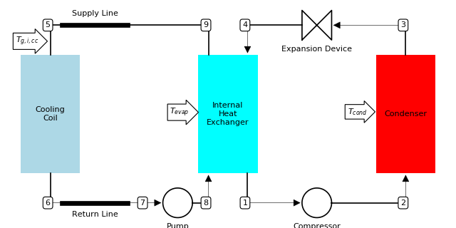
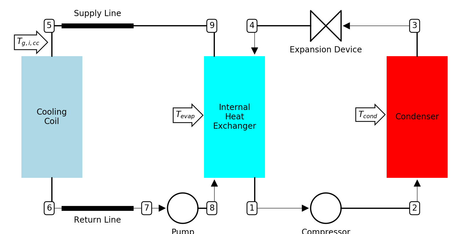
For secondary loops in cooling mode, there is an internal heat exchanger which physically separates the secondary loop and the refrigerant loop.
In this case, there are now three inputs, and three residuals (to be defined later). The three inputs are \(T_{g,i,cc}\), \(T_{evap}\) and \(T_{cond}\).
The two loops can be solved separately, where for the secondary loop, the inlet temperature to the cooling coil is known, and the secondary working fluid’s properties are independent of pressure.
To begin, the Cooling Coil model is employed to calculate the heat transfer rate in the cooling coil, which gives the process from state point 5 to state point 6.
The Line Set model is used to determine the heat transfer and pressure drop in the line going from state point 6 to state point 7.
The pump model is run to determine how much electrical power is consumed in the pump, which gives the state point 8, the glycol inlet to the internal heat exchanger.
The refrigerant loop is then solved. The refrigerant superheat at the outlet of the IHX is imposed as an input for the cycle. Thus state point 1 is known, and the Compressor model is used to calculate state point 2, the compressor mass flow rate, electrical power, etc..
The Condenser model is then solved using the state point 2 as the inlet, and yielding the (hopefully) subcooled refrigerant outlet state point 3.
Finally, the isenthalpic throttling process is used to determine the state point 4 at the refrigerant inlet to the IHX.
Lastly, the Plate-Heat-Exchangers model is run, using the inputs at state points 8 and 4, and yielding the refrigerant outlet state of state point 1’.
The residuals are given by an energy balance between state points 1 and 1’, an energy balance on the secondary loop, and either matching the mass or the subcooling on the refrigerant side. As in the DX system analysis, the residual vector is given by
with
The set of \(T_{g,i,cc}\), \(T_{evap}\) and \(T_{cond}\) which solve the residual equations are obtained by a multi-dimensional solver (see Multi-dimensional solver).
The common metrics of system efficiency are
from __future__ import print_function

from ACHP.Cycle import SecondaryCycleClass

# Instantiate the class
Cycle = SecondaryCycleClass()

#--------------------------------------
#       Cycle parameters
#--------------------------------------
Cycle.Verbosity = 0 #the idea here is to have different levels of debug output
Cycle.ImposedVariable = 'Subcooling' #or this could be 'Charge' for imposed charge
Cycle.DT_sc_target = 7.0
#Cycle.Charge_target = 2.4  #Needed if charge is imposed, not otherwise
Cycle.Ref='R410A'
Cycle.SecLoopFluid = 'MEG'
Cycle.MassFrac_SLF = 0.21 #Mass fraction of incompressible SecLoopFluid [i.e MEG-20%]
Cycle.Backend_SLF = 'INCOMP' #backend of SecLoopFluid
Cycle.IHXType = 'PHE'# or could be 'Coaxial'
Cycle.Mode='AC'

#--------------------------------------
#--------------------------------------
#       Compressor parameters
#--------------------------------------
#--------------------------------------

# A 3 ton cooling capacity compressor map
if Cycle.Ref=='R410A':
    M=[217.3163128,5.094492028,-0.593170311,4.38E-02,-2.14E-02,1.04E-02,
    7.90E-05,-5.73E-05,1.79E-04,-8.08E-05]
    P=[-561.3615705,-15.62601841,46.92506685,-0.217949552,0.435062616,
    -0.442400826,2.25E-04,2.37E-03,-3.32E-03,2.50E-03]

params={
    'M':M,
    'P':P,
    'Ref':Cycle.Ref,    #refrigerant
    'fp':0.15, #Fraction of electrical power lost as heat to ambient
    'Vdot_ratio': 1.0, #Displacement Scale factor to up- or downsize compressor (1=original)
    'Verbosity': 0, # How verbose should the debugging statements be [0 to 10]
  }
Cycle.Compressor.Update(**params)

#--------------------------------------
#      Condenser parameters
#--------------------------------------
Cycle.Condenser.Fins.Tubes.NTubes_per_bank=24  #number of tubes per bank=row
Cycle.Condenser.Fins.Tubes.Nbank=1             #number of banks/rows
Cycle.Condenser.Fins.Tubes.Ncircuits=3
Cycle.Condenser.Fins.Tubes.Ltube=2.252
Cycle.Condenser.Fins.Tubes.OD=0.00913
Cycle.Condenser.Fins.Tubes.ID=0.00849
Cycle.Condenser.Fins.Tubes.Pl=0.0191  #distance between center of tubes in flow direction
Cycle.Condenser.Fins.Tubes.Pt=0.0254  #distance between center of tubes orthogonal to flow direction

Cycle.Condenser.Fins.Fins.FPI=25      #Number of fins per inch
Cycle.Condenser.Fins.Fins.Pd=0.001    #2* amplitude of wavy fin
Cycle.Condenser.Fins.Fins.xf=0.001    #1/2 period of fin
Cycle.Condenser.Fins.Fins.t=0.00011   #Thickness of fin material
Cycle.Condenser.Fins.Fins.k_fin=237   #Thermal conductivity of fin material

Cycle.Condenser.Fins.Air.Vdot_ha=1.7934 #rated volumetric flowrate
Cycle.Condenser.Fins.Air.Tmean=308.15
Cycle.Condenser.Fins.Air.Tdb=308.15     #Dry Bulb Temperature
Cycle.Condenser.Fins.Air.p=101325       #Air pressure
Cycle.Condenser.Fins.Air.RH=0.51        #Relative Humidity
Cycle.Condenser.Fins.Air.RHmean=0.51
Cycle.Condenser.Fins.Air.FanPower=260

Cycle.Condenser.FinsType = 'WavyLouveredFins' #WavyLouveredFins, HerringboneFins, PlainFins
Cycle.Condenser.Ref=Cycle.Ref
Cycle.Condenser.Verbosity=0

#--------------------------------------
#      Cooling Coil parameters
#--------------------------------------
Cycle.CoolingCoil.Fins.Tubes.NTubes_per_bank=32
Cycle.CoolingCoil.Fins.Tubes.Nbank=3
Cycle.CoolingCoil.Fins.Tubes.Ncircuits=5
Cycle.CoolingCoil.Fins.Tubes.Ltube=0.452
Cycle.CoolingCoil.Fins.Tubes.OD=0.00913
Cycle.CoolingCoil.Fins.Tubes.ID=0.00849
Cycle.CoolingCoil.Fins.Tubes.Pl=0.0191
Cycle.CoolingCoil.Fins.Tubes.Pt=0.0254

Cycle.CoolingCoil.Fins.Fins.FPI=14.5
Cycle.CoolingCoil.Fins.Fins.Pd=0.001
Cycle.CoolingCoil.Fins.Fins.xf=0.001
Cycle.CoolingCoil.Fins.Fins.t=0.00011
Cycle.CoolingCoil.Fins.Fins.k_fin=237

Cycle.CoolingCoil.Fins.Air.Vdot_ha=0.56319
Cycle.CoolingCoil.Fins.Air.Tmean=297.039
Cycle.CoolingCoil.Fins.Air.Tdb=297.039
Cycle.CoolingCoil.Fins.Air.p=101325
Cycle.CoolingCoil.Fins.Air.RH=0.5
Cycle.CoolingCoil.Fins.Air.RHmean=0.5
Cycle.CoolingCoil.Fins.Air.FanPower=438

params={
    'Ref_g': Cycle.SecLoopFluid,
    'Backend_g': Cycle.Backend_SLF,
    'MassFrac_g': Cycle.MassFrac_SLF,
    'pin_g': 200,
    'Verbosity':0,
    'mdot_g':0.38,
    'FinsType':'WavyLouveredFins' #WavyLouveredFins, HerringboneFins, PlainFins
}
Cycle.CoolingCoil.Update(**params)

params={
    'ID_i':0.0278,
    'OD_i':0.03415,
    'ID_o':0.045,
    'L':50,
    'pin_g':300,
    'Ref_r':Cycle.Ref,
    'Ref_g':Cycle.SecLoopFluid,
    'Backend_g': Cycle.Backend_SLF,
    'MassFrac_g': Cycle.MassFrac_SLF,
    'Verbosity':0
    }
Cycle.CoaxialIHX.Update(**params)

params={
    'pin_h':300000,
    'Ref_h':Cycle.SecLoopFluid,
    'Backend_h': Cycle.Backend_SLF,
    'MassFrac_h': Cycle.MassFrac_SLF,
    'Ref_c':Cycle.Ref,

    #Geometric parameters
    'Bp' : 0.117,
    'Lp' : 0.300, #Center-to-center distance between ports
    'Nplates' : 46,
    'PlateAmplitude' : 0.001, #[m]
    'PlateThickness' : 0.0003, #[m]
    'PlateConductivity' : 15.0, #[W/m-K]
    'PlateWavelength' : 0.00628, #[m]
    'InclinationAngle' : 3.14159/3,#[rad]
    'MoreChannels' : 'Hot', #Which stream gets the extra channel, 'Hot' or 'Cold'
    'Verbosity':0,
    'DT_sh':5
}
Cycle.PHEIHX.Update(**params)

params={
    'eta':0.5,  #Pump+motor efficiency
    'mdot_g':0.38, #Flow Rate kg/s
    'pin_g':300000,
    'Ref_g':Cycle.SecLoopFluid,
    'Backend_g': Cycle.Backend_SLF,
    'MassFrac_g': Cycle.MassFrac_SLF,
    'Verbosity':0,
    }
Cycle.Pump.Update(**params)

params={
    'L':5,
    'k_tube':0.19,
    't_insul':0.02,
    'k_insul':0.036,
    'T_air':297,
    'Ref': Cycle.SecLoopFluid,
    'Backend': Cycle.Backend_SLF,
    'MassFrac': Cycle.MassFrac_SLF,
    'pin': 300000,
    'h_air':0.0000000001,
}

Cycle.LineSetSupply.Update(**params)
Cycle.LineSetReturn.Update(**params)
Cycle.LineSetSupply.OD=0.009525
Cycle.LineSetSupply.ID=0.007986
Cycle.LineSetReturn.OD=0.01905
Cycle.LineSetReturn.ID=0.017526

#Now solve
from time import time
t1=time()
Cycle.PreconditionedSolve()

#Outputs
print('Took '+str(time()-t1)+' seconds to run Cycle model')
print('Cycle coefficient of system performance is '+str(Cycle.COSP))
print('Cycle refrigerant charge is '+str(Cycle.Charge)+' kg')
which should yield the output, when run, of
Took 10.33457088470459 seconds to run Cycle model
Cycle coefficient of system performance is 2.7891650414848344
Cycle refrigerant charge is 1.4989869734994357 kg
Secondary Loop Heating Mode
This section is left intentionally empty
Cycle Solver Class Documentation
-
class
ACHP.Cycle.SecondaryCycleClass[source]¶ -
Calculate(DT_evap, DT_cond, Tin_CC)[source]¶ Inputs are differences in temperature [K] between HX air inlet temperature and the dew temperature for the heat exchanger.
- Required Inputs:
- DT_evap:
- Difference in temperature [K] between cooling coil air inlet temperature and refrigerant dew temperature
- DT_cond:
- Difference in temperature [K] between condenser air inlet temperature and refrigerant dew temperature
- Tin_CC:
- Inlet “glycol” temperature to line set feeding cooling coil
-
Nomenclature
| Variable | Description |
|---|---|
| \(COP\) | Coefficient of Performance [-] |
| \(COSP\) | Coefficient of System Performance [-] |
| \(h_1\) | Enthalpy at outlet of evaporator [J/kg] |
| \(h_{1'}\) | Enthalpy after going around the cycle [J/kg] |
| \(\dot m_r\) | Refrigerant mass flow rate [kg/s] |
| \(m_r\) | Model-predicted charge [kg] |
| \(m_{r,target}\) | Target refrigerant charge in system [kg] |
| \(T_{cond}\) | Condensing (dewpoint) temperature [K] |
| \(T_{evap}\) | Evaporating (dewpoint) temperature [K] |
| \(T_{g,i,cc}\) | Glycol inlet temperature to cooling coil [K] |
| \(\Delta T_{sh}\) | IHX outlet superheat [K] |
| \(\Delta T_{sc,cond}\) | Condenser outlet subcooling [K] |
| \(\Delta T_{sc,cond,target}\) | Condenser outlet subcooling target [K] |
| \(\dot Q_{cc}\) | Cooling coil heat transfer rate [W] |
| \(\dot W_{fan,cc}\) | Cooling coil fan power [W] |
| \(\dot W_{fan,cond}\) | Condenser fan power [W] |
| \(\dot W_{comp}\) | Compressor power input [W] |
| \(\vec \Delta\) | Residual vector [varied] |